Introduction

Natural Language Processing (NLP) is a rapidly growing field of artificial intelligence. Being able to understand, generate and translate text effectively are challenges that open the way to many technological advances. For a long time, Long Short-Term Memory5 (LSTM) based on Recurrent Neural Networks (RNN) were the dominant approach for sequential modeling of language data. LSTMs are better than traditional RNNs at retaining information over long sequences thanks to their gate mechanism. However, their ability to effectively capture very long-range contextual dependencies remains limited. It is in this context that the Transformer model appeared in 2017, proposed by a team of Google researchers. Rather than using a recurrent structure, Transformers incorporate an attention mechanism allowing them to learn the contextual dependencies between elements in a sequence. This revolutionary architecture very quickly surpassed RNNs on many NLP tasks such as machine translation. Since then, Transformers have become omnipresent in the field. Giant models such as BERT or GPT-3 have enabled major advances in understanding and generating text. However, many questions remain open about their complex inner workings. In this article, we present in detail the Transformer architecture as well as its current applications.

Sequentials models of NLP

What is RNN?

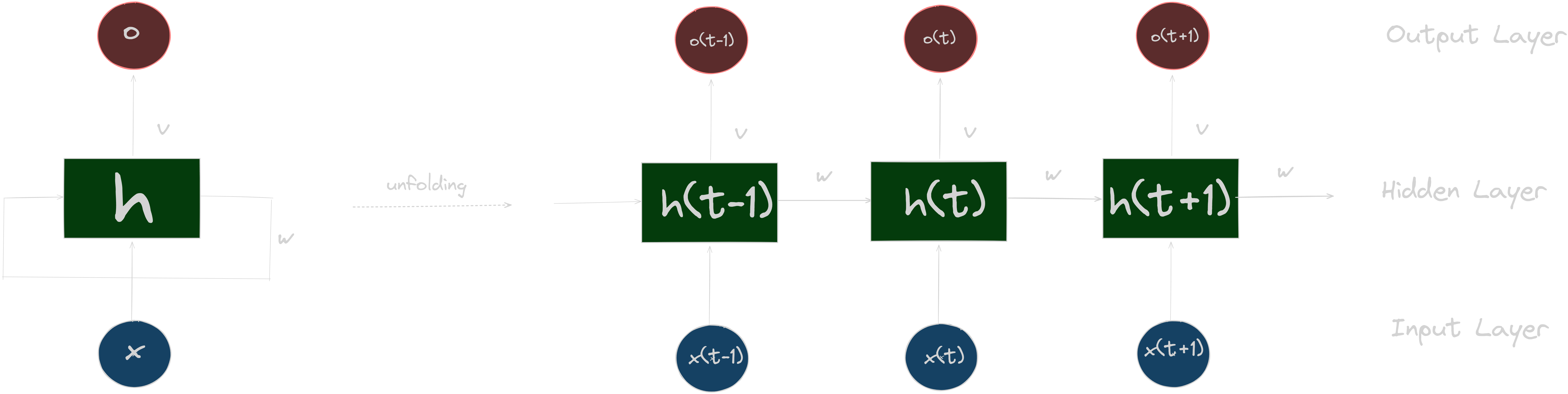
Recurrent neural networks (RNN) are models specialized in the analysis of sequential data such as text or speech. Unlike traditional networks which only see information isolated from each other, RNNs are able to memorize what they have already seen thanks to their internal memory. This memory, called hidden state, keeps track of the previous context at each stage of processing a sequence. So when the RNN looks at a new element, it also remembers the previous ones thanks to its hidden state. This is what allows RNNs to efficiently analyze data like sentences or music, where the order of words/sounds is important. Rather than seeing everything separately, the RNN understands how each part fits together. Thanks to their dynamic internal memory, RNNs are today widely used in language and speech processing by machines. It is one of the key tools to teach them to communicate better with us. The figure below represent a global architecture of RNN where x, h, o are the input sequence, hidden state and output sequence respectively. U, V and W are the training weights.

However, they face a limitation called the vanishing gradient problem. Indeed, when an RNN processes the elements of a sequence one after the other, the influence of the first elements analyzed tends to fade over time. It’s as if the network has more and more difficulty remembering the beginning of the sequence as it goes on. Then, LSTM model come to resolve it.

What is LSTM ?

LSTM is a specific type of RNN architecture that addresses the vanishing gradient problem, which occurs when training deep neural networks. LSTMs leverage memory cells and gates to selectively store and retrieve information over long sequences, making them effective at capturing long-term dependencies. The figure blow shows a memory cell architecture of LSTM model:

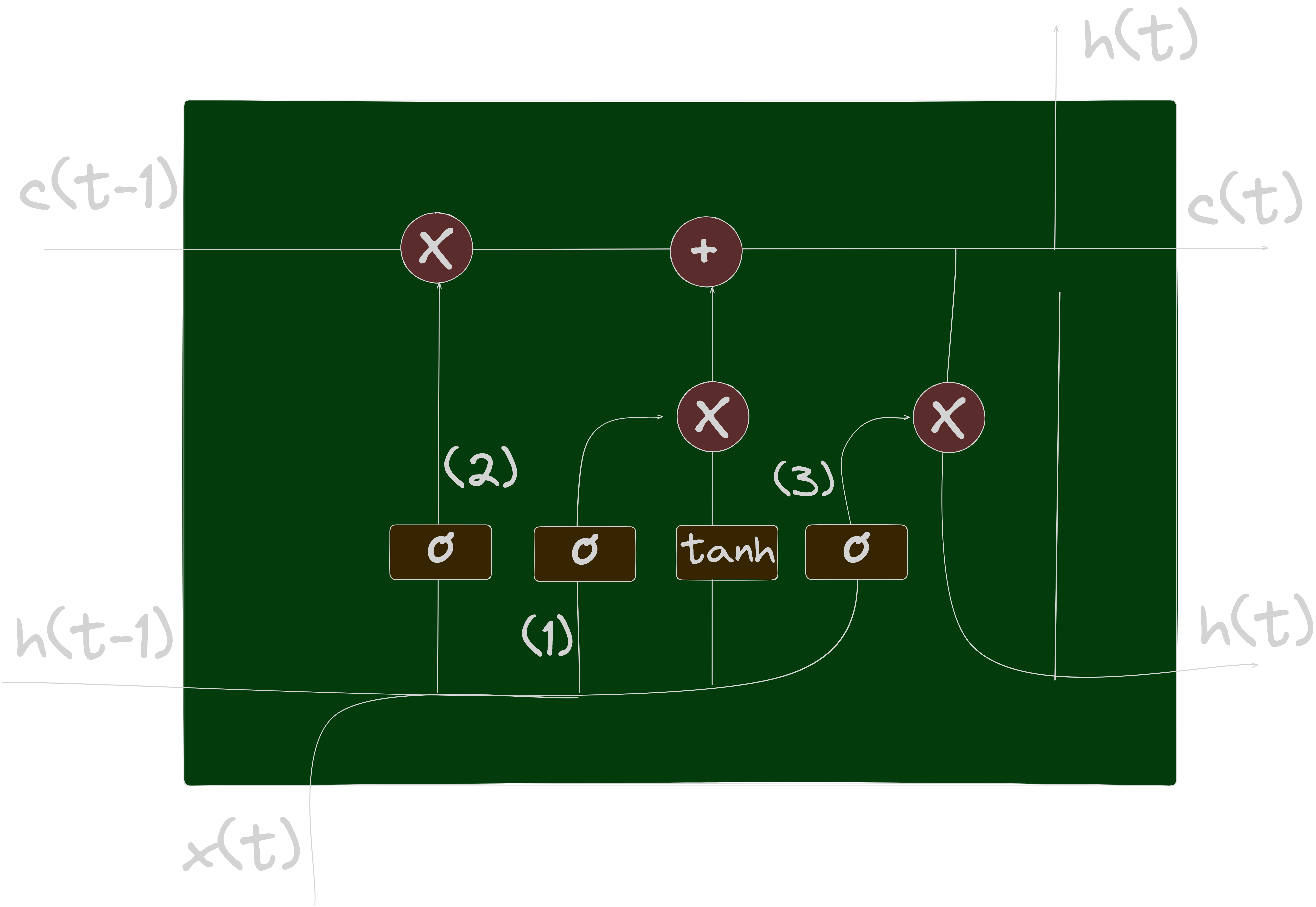
LSTMs have a memory cell allowing them to better manage long-term dependencies. This memory cell is made up of three gates:

The input gate
The forget gate
The output gate

These gates regulate the flow of information inside the memory cell, thus making it possible to control what information is remembered and what information is forgotten. This gives LSTM the ability to remember important information over long sequences and ignore less relevant material. $h_t$ is the usual hidden state of RNNs but in LSTM networks we add a second state called $c_t$ . Here, $h_t$ represents the neuron’s short memory (previous word) and $c_t$ represents the long-term memory (all the previous words history).

Forget gate

This gate decides what information must be kept or discarded: the information from the previous hidden state is concatenated to the input data (for example the word “des” vectorized) then the sigmoid function is applied to it in order to normalize the values between 0 and 1. If the output of the sigmoid is close to 0, this means that we must forget the information and if it is close to 1 then we must memorize it for the rest.

Input gate

The role of the entry gate is to extract information from the current data (the word “des” for example): we will apply in parallel a sigmoid to the two concatenated data (see previous gate) and a tanh.

Sigmoid (on the blue circle) will return a vector for which a coordinate close to 0 means that the coordinate in the equivalent position in the concatenated vector is not important. Conversely, a coordinate close to 1 will be deemed “important” (i.e. useful for the prediction that the LSTM seeks to make).
Tanh (on the red circle) will simply normalize the values (overwrite them) between -1 and 1 to avoid problems with overloading the computer with calculations.
The product of the two will therefore allow only the important information to be kept, the others being almost replaced by 0.

Cell state

We talk about the state of the cell before approaching the last gate (output gate), because the value calculated here is used in it. The state of the cell is calculated quite simply from the oblivion gate and the entry gate: first we multiply the exit from oblivion coordinate by coordinate with the old state of the cell. This makes it possible to forget certain information from the previous state which is not used for the new prediction to be made. Then, we add everything (coordinate to coordinate) with the output of the input gate, which allows us to record in the state of the cell what the LSTM (among the inputs and the previous hidden state) has deemed relevant.

Output gate

Last step: the output gate must decide what the next hidden state will be, which contains information about previous inputs to the network and is used for predictions. To do this, the new state of the cell calculated just before is normalized between -1 and 1 using tanh. The concatenated vector of the current input with the previous hidden state passes, for its part, into a sigmoid function whose goal is to decide which information to keep (close to 0 means that we forget, and close to 1 that we will keep this coordinate of the state of the cell). All this may seem like magic in the sense that it seems like the network has to guess what to retain in a vector on the fly, but remember that a weight matrix is applied as input. It is this matrix which will, concretely, store the fact that such information is important or not based on the thousands of examples that the network will have seen!

What is a Transformer?

The Transformer is a neural network architecture proposed in the seminal paper “Attention Is All You Need” by Vaswani et al. Unlike RNNs, Transformers do not rely on recurrence but instead operate on self-attention. Self-attention allows the model to weigh the importance of different input tokens when making predictions, enabling it to capture long-range dependencies without the need for sequential processing. Transformers consist of encoder and decoder layers, employing multi-head self-attention mechanisms and feed-forward neural networks. The figure below shows the architecture of a Transformer network:

From LSTM to transformers

Neural networks are very efficient statistical models for analyzing complex data with variable formats. If models like CNNs emerged for processing visual data, for text processing, the neural network architectures that were used were RNNs, and more particularly LSTMs.

LSTMs make it possible to resolve one of the major limitations of classic neural networks: they make it possible to introduce a notion of context, and to take into account the temporal component. This is what made them popular for language processing. Instead of analyzing words one by one, we could analyze sentences in a very specific context. However, LSTMs, and RNNs in general, did not solve all the problems.

First, their memory is too short to be able to process paragraphs that are too long
Then, RNNs process data sequentially, and are therefore difficult to parallelize. Except that the best language models today are all characterized by an astronomical amount of data. Training an LSTM model using the data consumed by GPT-3 would have taken decades.

This is where Transformers come in, to revolutionize deep learning. They were initially proposed for translation tasks. And their major characteristic is that they are easily parallelizable. Which makes training on huge databases faster. For example, GPT-3 was trained on a database of over 45TB of text, almost the entire internet. They have made it possible to achieve unprecedented levels of performance on tasks such as translation or image generation and are the basis of what we today call generative artificial intelligence.

Let’s study GPT transfomer architecture😊

Transformer architecture of GPT model

In this diagram, the data flows from the bottom to the top, as is traditional in Transformer illustrations. Initially, our input tokens undergo several encoding steps:

They are encoded using an Embedding layer. This assigns a unique vector representation to each input token.
They then pass through a Positional Encoding layer. This encodes positional information by adding signals to the embedding vectors.
The output of the Embedding layer and Positional Encoding layer are added together. This combines the token representation with its positional context.

Next, the encoded inputs go through a sequence of N decoding steps. Each decoding step processes the encoded inputs using self-attention and feedforward sublayers. Finally, the decoded data is processed in two additional steps:

It passes through a normalization layer to regulate the output scale.
It is then sent through a linear layer and softmax. This produces a probability distribution over possible next tokens that can be used for prediction.

In the sections that follow, we’ll take a closer look at each of the components in this architecture.

Embedding

The Embedding layer turns each token in the input sequence into a vector of length d_model. The input of the Transformer consists of batches of sequences of tokens, and has shape (batch_size, seq_len). The Embedding layer takes each token, which is a single number, calculates its embedding, which is a sequence of numbers of length d_model, and returns a tensor containing each embedding in place of the corresponding original token. Therefore, the output of this layer has shape (batch_size, seq_len, d_model).

import torch.nn as nn

class Embeddings(nn.Module):
	def __init__(self, d_model, vocab_size): 
		super(Embeddings, self).__init__() 
		self.lut = nn.Embedding(vocab_size, d_model)
		self.d_model = d_model 
		# input x: (batch_size, seq_len) 
		# output: (batch_size, seq_len, d_model) 
	def forward(self, x): 
		out = self.lut(x) * math.sqrt(self.d_model) 
		return out

The purpose of using an embedding instead of the original token is to ensure that we have a similar mathematical vector representation for tokens that are semantically similar. For example, let’s consider the words “she” and “her”. These words are semantically similar, in the sense that they both refer to a woman or girl, but the corresponding tokens can be completely different (for example, when using OpenAI’s tiktoken tokenizer, “she” corresponds to token 7091, and “her” corresponds to token 372). The embeddings for these two tokens will start out being very different from one another as well, because the weights of the embedding layer are initialized randomly and learned during training. But if the two words frequently appear nearby in the training data, eventually the embedding representations will converge to be similar.

Positional Encoding

The Positional Encoding layer adds information about the absolute position and relative distance of each token in the sequence. Unlike recurrent neural networks (RNNs) or convolutional neural networks (CNNs), Transformers don’t inherently possess any notion of where in the sequence each token appears. Therefore, to capture the order of tokens in the sequence, Transformers rely on a Positional Encoding.

There are many ways to encode the positions of tokens. For example, we could implement the Positional Encoding layer by using another embedding module (similar to the previous layer), if we pass the position of each token rather than the value of each token as input. Once again, we would start with the weights in this embedding chosen randomly. Then during the training phase, the weights would learn to capture the position of each token.

class PositionalEncoding(nn.Module):
	def __init__(self, d_model, dropout, max_len=5000):
		super(PositionalEncoding, self).__init__()
		self.dropout = nn.Dropout(p=dropout)
		pe = torch.zeros(max_len, d_model) 
		position = torch.arange(0, max_len).unsqueeze(1) # (max_len, 1) 
		div_term = torch.exp( torch.arange(0, d_model, 2) * -(math.log(10000.0) / d_model)) # (d_model/2) 
		pe[:, 0::2] = torch.sin(position * div_term) # (max_len, d_model)
		pe[:, 1::2] = torch.cos(position * div_term) # (max_len, d_model)
		pe = pe.unsqueeze(0) # (1, max_len, d_model)
		self.register_buffer('pe', pe)
	 
	# input x: (batch_size, seq_len, d_model) 
	# output: (batch_size, seq_len, d_model) 
	def forward(self, x):
		x = x + Variable(self.pe[:, :x.size(1)], requires_grad=False) 
		return self.dropout(x)

Decoder

As we saw in the diagrammatic overview of the Transformer architecture, the next stage after the Embedding and Positional Encoding layers is the Decoder module. The Decoder consists of N copies of a Decoder Layer followed by a Layer Norm. Here’s the Decoder class, which takes a single DecoderLayer instance as input to the class initializer:

class Decoder(nn.Module): 
	def __init__(self, layer, N): 
		super(Decoder, self).__init__() 
		self.layers = clones(layer, N) 
		self.norm = LayerNorm(layer.size) 
	def forward(self, x, mask): 
		for layer in self.layers: 
			x = layer(x, mask) 
		return self.norm(x)

The Layer Norm takes an input of shape (batch_size, seq_len, d_model) and normalizes it over its last dimension. As a result of this step, each embedding distribution will start out as unit normal (centered around zero and with standard deviation of one). Then during training, the distribution will change shape as the parameters a_2 and b_2 are optimized for our scenario.

class LayerNorm(nn.Module): 
	def __init__(self, features, eps=1e-6): 
		super(LayerNorm, self).__init__() 
		self.a_2 = nn.Parameter(torch.ones(features)) 
		self.b_2 = nn.Parameter(torch.zeros(features)) 
		self.eps = eps 
	def forward(self, x): 
		mean = x.mean(-1, keepdim=True) 
		std = x.std(-1, keepdim=True) 
		return self.a_2 * (x - mean) / (std + self.eps) + self.b_2

The DecoderLayer class that we clone has the following architecture:

decoder layer

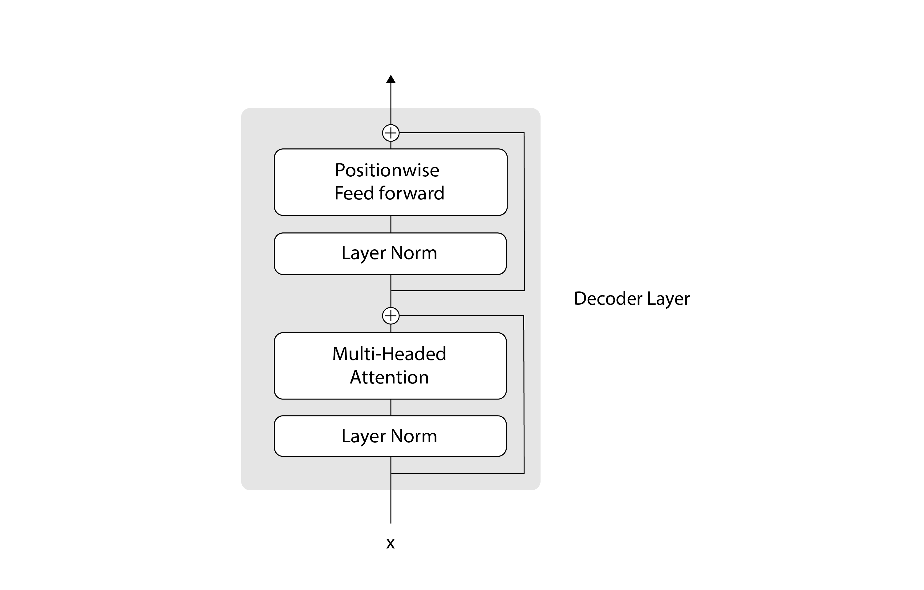
Here’s the corresponding code:

class DecoderLayer(nn.Module): 
	def __init__(self, size, self_attn, feed_forward, dropout):
	super(DecoderLayer, self).__init__() 
	self.size = size 
	self.self_attn = self_attn 
	self.feed_forward = feed_forward 
	self.sublayer = clones(SublayerConnection(size, dropout), 2) 
	def forward(self, x, mask): 
		x = self.sublayer[0](x, lambda x: self.self_attn(x, x, x, mask)) 
		return self.sublayer[1](x, self.feed_forward)

At a high level, a DecoderLayer consists of two main steps:

The attention step, which is responsible for the communication between tokens
The feed forward step, which is responsible for the computation of the predicted tokens.

Surrounding each of those steps, we have residual (or skip) connections, which are represented by the plus signs in the diagram. Residual connections provide an alternative path for the data to flow in the neural network, which allows skipping some layers. The data can flow through the layers within the residual connection, or it can go directly through the residual connection and skip the layers within it. In practice, residual connections are often used with deep neural networks, because they help the training to converge better. You can learn more about residual connections in the paper Deep residual learning for image recognition, from 2015. We implement these residual connections using the SublayerConnection module:


class SublayerConnection(nn.Module): 
	def __init__(self, size, dropout): 
		super(SublayerConnection, self).__init__() 
		self.norm = LayerNorm(size) 
		self.dropout = nn.Dropout(dropout) 
	def forward(self, x, sublayer): 
		return x + self.dropout(sublayer(self.norm(x)))

The feed-forward step is implemented using two linear layers with a Rectified Linear Unit (ReLU) activation function in between:


class PositionwiseFeedForward(nn.Module):

    def __init__(self, d_model, d_ff, dropout=0.1):
        super(PositionwiseFeedForward, self).__init__()
        self.w_1 = nn.Linear(d_model, d_ff)
        self.w_2 = nn.Linear(d_ff, d_model)
        self.dropout = nn.Dropout(dropout)

    def forward(self, x):
        return self.w_2(self.dropout(F.relu(self.w_1(x))))

The attention step is the most important part of the Transformer, so we’ll devote the next section to it😊.

Masked multi-headed self-attention

The multi-headed attention section in the previous diagram can be expanded into the following architecture:

multi-headed self-attention

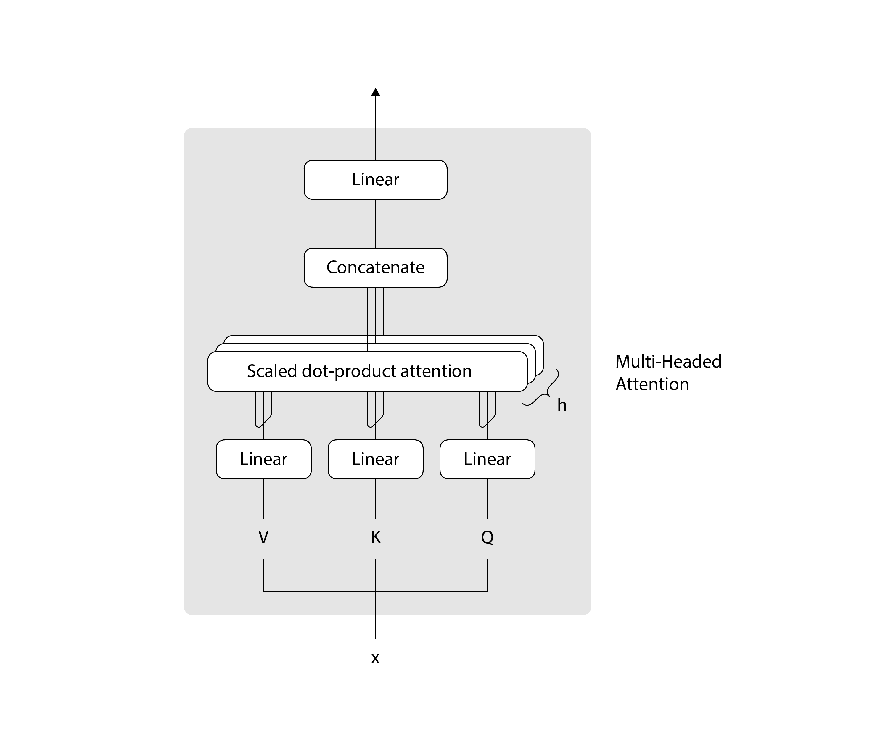
Each multi-head attention block is made up of four consecutive levels:

On the first level, three linear (dense) layers that each receive the queries, keys, or values
On the second level, a scaled dot-product attention function. The operations performed on both the first and second levels are repeated h times and performed in parallel, according to the number of heads composing the multi-head attention block.
On the third level, a concatenation operation that joins the outputs of the different heads
On the fourth level, a final linear (dense) layer that produces the output

Recall as well the important components that will serve as building blocks for your implementation of the multi-head attention:

The queries, keys, and values: These are the inputs to each multi-head attention block. In the encoder stage, they each carry the same input sequence after this has been embedded and augmented by positional information. Similarly, on the decoder side, the queries, keys, and values fed into the first attention block represent the same target sequence after this would have also been embedded and augmented by positional information. The second attention block of the decoder receives the encoder output in the form of keys and values, and the normalized output of the first decoder attention block as the queries. The dimensionality of the queries and keys is denoted by d(k), whereas the dimensionality of the values is denoted by d(v).
The projection matrices: When applied to the queries, keys, and values, these projection matrices generate different subspace representations of each. Each attention head then works on one of these projected versions of the queries, keys, and values. An additional projection matrix is also applied to the output of the multi-head attention block after the outputs of each individual head would have been concatenated together. The projection matrices are learned during training.

Generator

The last step in our Transformer is the Generator, which consists of a linear layer and a softmax executed in sequence:

class Generator(nn.Module): 
	def __init__(self, d_model, vocab): 
		super(Generator, self).__init__() 
		self.proj = nn.Linear(d_model, vocab) 
	def forward(self, x): 
		return F.log_softmax(self.proj(x), dim=-1)

The purpose of the linear layer is to convert the third dimension of our tensor from the internal-only d_model embedding dimension to the vocab_size dimension, which is understood by the code that calls our Transformer. The result is a tensor dimension of (batch_size, seq_len, vocab_size). The purpose of the softmax is to convert the values in the third tensor dimension into a probability distribution. This tensor of probability distributions is what we return to the user.

You might remember that at the very beginning of this article, we explained that the input to the Transformer consists of batches of sequences of tokens, of shape (batch_size, seq_len). And now we know that the output of the Transformer consists of batches of sequences of probability distributions, of shape (batch_size, seq_len, vocab_size). Each batch contains a distribution that predicts the token that follows the first input token, another distribution that predicts the token that follows the first and second input tokens, and so on. The very last probability distribution of each batch enables us to predict the token that follows the whole input sequence, which is what we care about when doing inference.

The Generator is the last piece of our Transformer architecture, so we’re ready to put it all together. To know how to train and implement it all together.

Difference between RNNs and Transformers

Architecture

RNNs are sequential models that process data one element at a time, maintaining an internal hidden state that is updated at each step. They operate in a recurrent manner, where the output at each step depends on the previous hidden state and the current input.

Transformers are non-sequential models that process data in parallel. They rely on self-attention mechanisms to capture dependencies between different elements in the input sequence. Transformers do not have recurrent connections or hidden states.

Handling Sequence Length

RNNs can handle variable-length sequences as they process data sequentially. However, long sequences can lead to vanishing or exploding gradients, making it challenging for RNNs to capture long-term dependencies.

Transformers can handle both short and long sequences efficiently due to their parallel processing nature. Self-attention allows them to capture dependencies regardless of the sequence length.

Dependency Modeling

RNNs are well-suited for modeling sequential dependencies. They can capture contextual information from the past, making them effective for tasks like language modeling, speech recognition, and sentiment analysis.

Transformers excel at modeling dependencies between elements, irrespective of their positions in the sequence. They are particularly powerful for tasks involving long-range dependencies, such as machine translation, document classification, and image captioning.

Size of the Model

The size of an RNN is primarily determined by the number of recurrent units (e.g., LSTM cells or GRU cells) and the number of parameters within each unit. RNNs have a compact structure as they mainly rely on recurrent connections and relatively small hidden state dimensions. The number of parameters in an RNN is directly proportional to the number of recurrent units and the size of the input and hidden state dimensions.

Transformers tend to have larger model sizes due to their architecture. The main components contributing to the size of a Transformer model are self-attention layers, feed-forward layers, and positional encodings. Transformers have a more parallelizable design, allowing for efficient computation on GPUs or TPUs. However, this parallel processing capability comes at the cost of a larger number of parameters.

Training and Parallelisation

For RNN, we mostly train it in a sequential approach, as the hidden state relies on previous steps. This makes parallelization more challenging, resulting in slower training times.

On the other hand, we train Transformers in parallel since they process data simultaneously. This parallelization capability speeds up training and enables the use of larger batch sizes, which makes training more efficient.

Conclusion

In this article, we explain the basic idea behind RNN/LSTM and Transformer. Furthermore, we compare these two types of networks from multiple aspects. We also talked about the architecture of transformers in the GPT model. While RNNs and LSTMs were the go-to choices for sequential tasks, Transformers are proving to be a viable alternative due to their parallel processing capability, ability to capture long-range dependencies, and improved hardware utilization. . However, RNNs still have value when it comes to tasks where temporal dependencies play a critical role. In conclusion, the choice between RNN/LSTM and Transformer models ultimately depends on the specific requirements of the task at hand, striking a balance between efficiency, accuracy and interpretability.

Understanding the transformer architecture in NLP