Introduction

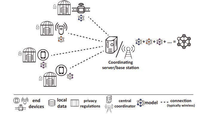
Federated learning is a promising machine learning technique that enables multiple clients to collaboratively build a model without revealing the raw data to each other. The standard implement of FL adopts the conventional parameter server architecture where end devices are connected to the central coordinator in a start topology. The coordinator can be a central server or a base station at the network edge. Compared to traditional distributed learning methods, the key features of FL are :

• No data sharing and the server stays agnostic of any training data
• Exchange of encrypted models instead of exposing gradients
• Sparing device-server communications instead of batch-wise gradient uploads Among various types of federated learning methods, horizontal federated learning (HFL) is the best-studied category and handles homogeneous feature spaces. The figure shows a typical cross-device FL scenario where a multitude of user devices are coordinated by a central server(at the edge or on the cloud). This article aims to show how horizontal federated learning can be applied to a dataset. I conducted experiments on various cases using CIFAR10 datasets and demonstrated that HFL can achieve excellent performance while ensuring the confidentiality of our data, making it a valuable tool for boosting model performance.

Architecture of HFL

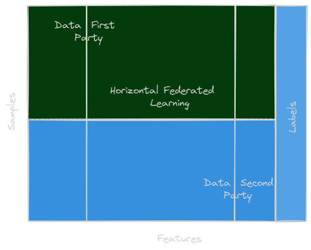
Horizontal federated learning was designed for training on distributed datasets that typically share the same feature space whilst having little or non overlap in terms of their data instances. It refers to building a model in the scenario where datasets have significant overlaps on the feature spaces($X_1$, $X_2$, …) but not on the ID spaces. The figure below show you a guidebook of HFL.

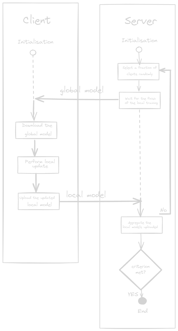
The standard process of FL is organised in rounds. After initialisation, each round is comprised of the following steps (the figure below show an illustration of this):

• The server selects a fraction of clients randomly to participate in this round of training.
• The server distributes the latest global model to the selected clients
• The selected clients download the global model to overwrite their local models and perform training on their local data to update the modes
• The selected clients upload their updated local models to the server
• The server agregates the local models from the clients into a new global model

The process repeats for a preset number of rounds or until the global model attains the desired level of quality (judged from the loss or accuracy in evaluations).

Experimental methodology

In the remainder of this article, we will delve deeper into the different aspects of horizontal federated learning by using Tensorflow Federated Learning algorithm(TFF). We have already discussed the basic structure of this process, where each client performs local training on classic machine learning models such as Decision Trees or Keras. Then, the parameters of these models are sent to the central server to be aggregated, creating a better performing overall model. This crucial step requires the choice of an optimal aggregation function in order to obtain the best possible precision. We will therefore discuss in detail the different aggregation functions used in the federated model, as well as the tests carried out to evaluate their performance. We will also present the datasets used during these tests and interpret the results obtained.

Additionally, training a federated model involves several essential compartments, such as client selection, client training, model aggregation, and updates. We will pay particular attention to these key components and discuss their role and importance in the federated learning process.

Finally, we will examine the different tests carried out to improve the accuracy of the federated model. We will analyze the results obtained by varying the hyperparameters and exploring different configurations. This step will allow us to understand how hyperparameter choices affect model performance and identify best practices to improve accuracies.

Aggregation functions of TFF model

Datasets

CIFAR-10 data is one of the most commonly used datasets in the field of computer vision and machine learning. They are widely used for evaluation and comparison of machine learning models in image classification tasks.

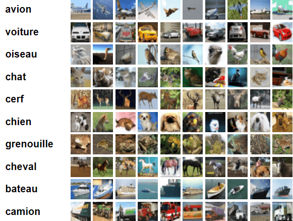
The CIFAR-10 data consists of a set of 60,000 color images of size 32x32 pixels. The images are divided into 10 different classes, with 6,000 images per class. Classes include: plane, automobile, bird, cat, deer, dog, frog, horse, ship and truck.

The CIFAR-10 dataset consists of 60,000 32 x 32 color images divided into 10 classes, with 6,000 images per class. There are 50,000 training images and 10,000 test images. The dataset is divided into five training batches and one testing batch, each containing 10,000 images. The test batch contains exactly 1000 randomly selected images from each class. Training batches contain the remaining images in random order, but some training batches may contain more images from one class than another. In total, the training batches contain exactly 5,000 images of each class.

The images are in RGB format (red, green, blue) and are represented as 3D matrices with a depth of 3 color channels. Each image is represented by a matrix of dimensions 32x32x3, where the three dimensions correspond to width, height and color channels respectively. Pixels in each color channel are represented by 8-bit unsigned integers, ranging from 0 to 255.

CIFAR-10 data is often used to train and evaluate image classification models, such as convolutional neural networks (CNN). These data are popular for classification tasks due to their diversity, complexity, and relatively small size. Model performance is typically evaluated in terms of classification accuracy on the test batch.

Aggregation functions

Evaluation of aggregate functions

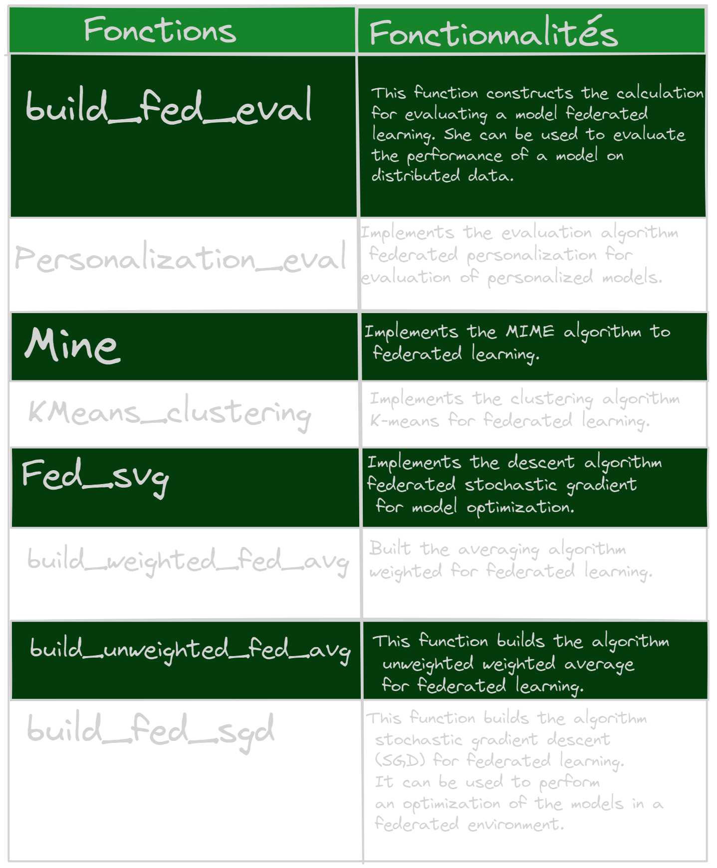
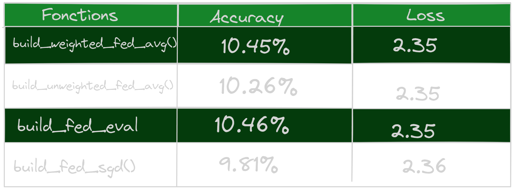
Federated models use different aggregation functions to combine updates from clients’ local models. In our case, we chose the following functions which are the most suitable for our needs: build_weighted_fed_avg(), build_unweighted_fed_avg(), build_fed_eval(), and build_fed_sgd(). Each of these aggregation functions has specific characteristics and can influence the performance of the overall model. It is therefore important to understand the specificities of the different functions in order to choose the most suitable function in your case.

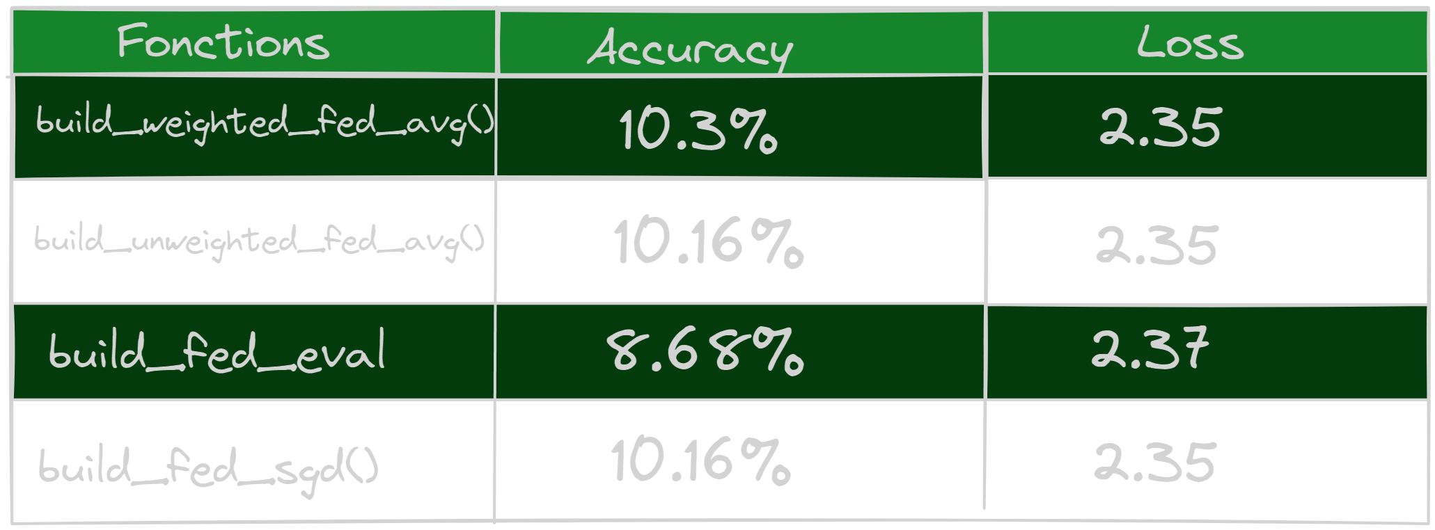
To evaluate the performance of the different aggregation functions, we carried out several tests. We varied the number of clients in each test in order to measure the impact of this parameter on the accuracies obtained. For each configuration, we noted the accuracy (correct classification rate) as well as the loss of the federated model. These metrics allow us to evaluate the quality of the model’s predictions and understand how performance varies depending on the number of customers.

By performing these tests, we aim to identify the aggregation function best suited to our specific use case. We seek to maximize the accuracies obtained while minimizing the loss of the federated model. By analyzing the results obtained, we will be able to determine which aggregation function offers the best performance in our particular context.

• Federated learning on 3 clients
• Federated learning on 5 clients
• Federated learning on 20 clients
• Federated learning on 50 clients
• Federated learning on 100 clients

Results analysis of tests

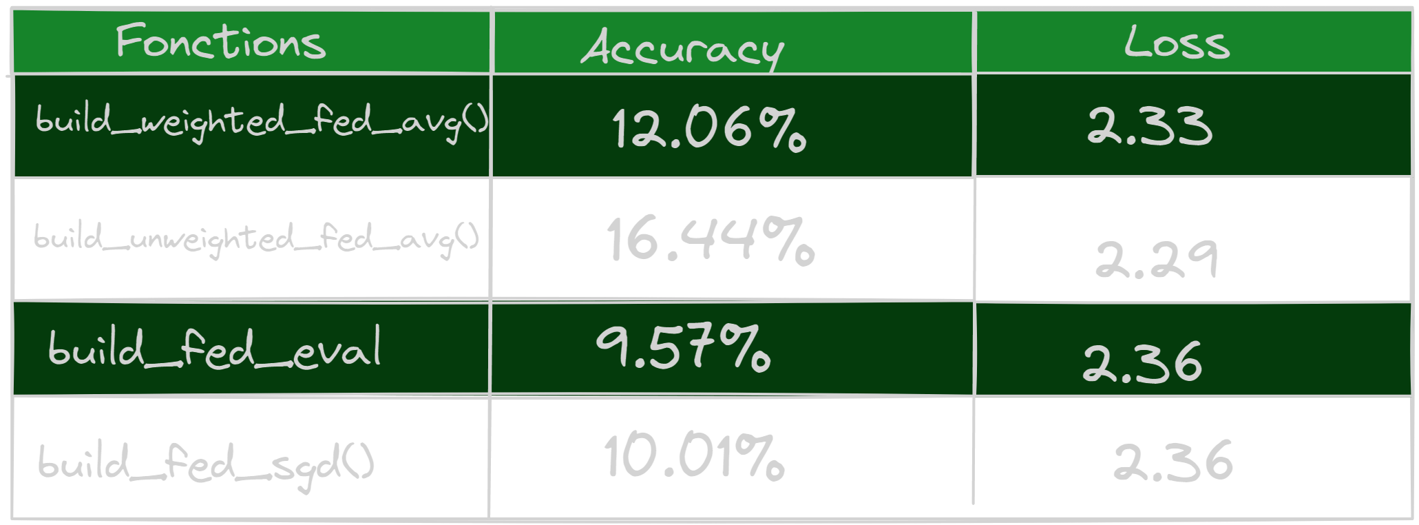
The study carried out revealed that the build_weighted_fed_avg() method performs better when used with any number of clients, resulting in better accuracy. This function sets up a federated average calculation process that integrates customer weights during the aggregation step. Client weights are typically determined based on specific criteria, such as the number of data points or the quality of the client’s data. This approach allows customer contributions to be weighted differently, placing greater importance on customers whose data is more representative or reliable.

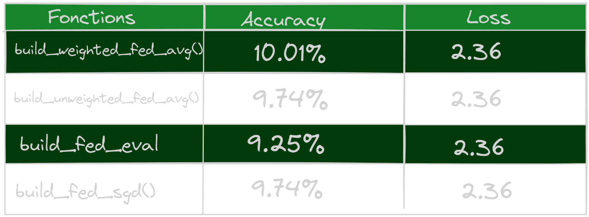
Additionally, another test was carried out using 100 clients, and it was observed that the accuracies obtained are even better. This can be explained by the fact that the higher the number of clients, the greater the chances of obtaining the best weights during aggregation. Indeed, by having a larger number of clients, it is possible to benefit from a greater diversity of data, which can improve the accuracy of the federated model. It is important to note that other criteria may also contribute to improving these accuracies, and these may vary depending on the specific context of the application.

Training components of TFF model

Identifying the components of TFF

During training, I identified the key components of the federated learning model, which are virtual or logical entities responsible for different parts of the federated learning process:

Client 1: client_work
Client 2: aggregator
Client 3: finalizer
Client 4: distributor

Role and importance of components

The different components listed above have specific roles to carry out the entire process of federative learning.

Customer 0: distributor The client distributor is a logical entity responsible for distributing the weights of the initial model to the different clients.

Client 1: client_work The term client generally refers to decentralized entities or devices (e.g. mobile devices, edge servers, etc.) that perform learning on their own local data. Each client performs local training on its data and then sends model updates to the central server (aggregator) for aggregation.

Client 2: aggregator The aggregator entity is responsible for aggregating model updates from different clients. It combines updates from multiple clients to get an overall model update. The aggregator can use different aggregation strategies, such as weighted average of client updates, to update the overall model.

Client 3: Finalizer The finalizer client is involved in some post-processing or validation steps after model aggregation. It can perform additional calculations, quality assessments, or final adjustments on the aggregated model before deploying it or making it available for future learning iterations.

Improved performance of TFF

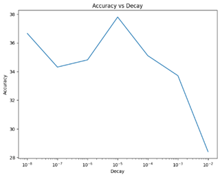
The training was carried out in two different cases. In the first case, the basic CNN model was used by clients to classify images. A set of hyperparameter values, such as learning rate and decay, was tested over 150 epochs to study the variation in accuracies and determine the best combinations. In a second case, the pre-trained model EfficientNet was used to compare the results using the CNN model. The graphs below illustrate these different variations.

By analyzing the graphs, we can observe changes in accuracy based on hyperparameter values. This allows us to choose the best performing combinations to optimize the model. Variations in accuracies give us indications on the sensitivity of the model to different hyperparameter settings.

Using these results, we can select the hyperparameter values ​​that lead to maximum accuracy for our base CNN model. This helps us fine-tune settings and improve model performance when classifying images.

NB: Learning rate: hyperparameter that determines the size of the steps that your learning algorithm takes when optimizing the model. In other words, it controls the speed at which your model learns.

Decay is a concept linked to the learning rate. This is a commonly used technique to gradually reduce the learning rate over time while training the model. Decay helps stabilize learning by adjusting the learning rate as training progresses.

Training on different hyperparameters

Using CNN model

• Variation of learning rate

• Variation of decay

Using EfficientNet model

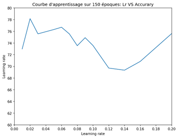
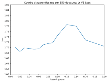
• Variation of learning rate -Variation of decay

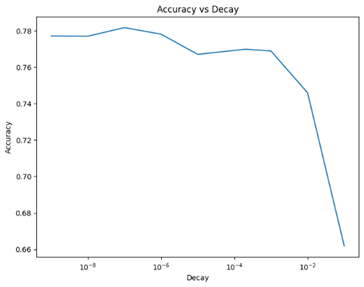
Results analysis

Using CNN model

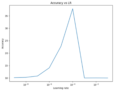
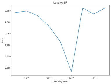
An increasing trend in accuracy can be observed as training progresses, but at a certain level it decreases significantly. Indeed, the accuracy is higher when the learning rate has a low value, but it decreases considerably when the learning rate is higher.

From the graph, we see that the smaller the decay, the higher the precision. The tests carried out demonstrated that optimal training is between 9% and 38% accuracy, which is considerably better than previously obtained results. However, it is possible that the accuracy remains static due to the low number of clients (5 clients). By increasing the number of customers, the results could be even better. It is also important to take into account that the CNN model may have difficulty adapting to a federated model.

Using EfficientNet model

The two tests revealed that the optimal values ​​of the learning rate are between 0.01 and 0.07, while those of the decay are between 0.001 and 1E-9, of the order of 1E-1. The maximum accuracy obtained is around 78%, which is significantly higher than the accuracy obtained with the CNN model.

It is interesting to note that the most optimal values ​​of learning rate and decay are generally low. This indicates that lower learning rates and decays promote better performance. The EfficientNet-based TFF model is found to be more optimal due to its ability to classify images accurately, thanks to its pre-training. Even better accuracies can be achieved by increasing the number of clients or further adjusting the parameters.

In summary, the test results suggest that lower values ​​of learning rate and decay lead to better accuracies. The EfficientNet-based TFF model, as a pre-trained model, provides better initial performance. To further improve results, it is recommended to explore configurations with larger numbers of clients or continue adjusting settings.

Conclusion

This article has explored in detail the different aspects of horizontal federated learning, including its definition, architecture, feasibility and case studies. We have seen that the federated learning model has many advantages, in particular the preservation of data confidentiality, while allowing good results in terms of precision.

The results of the tests carried out demonstrated that the use of the horizontal federated learning model, using techniques such as the TFF model based on EfficientNet, can lead to higher levels of accuracy than those obtained with traditional models such as the CNN. The optimal values ​​of learning rate and decay were identified, and it was found that lower values ​​of these hyperparameters promote better performance.

It is now worth emphasizing that the next research works focus on vertical federated learning, which is a different case from horizontal federated learning when it comes to data usage between clients. Vertical federated learning involves collaboration between clients with different but complementary data. This approach opens new perspectives for federated learning and requires in-depth study to optimize performance and data privacy in this context.