Deep Learning and Recurrent Neural Networks (RNNs)

Deep learning has made significant strides in recent years, transforming various fields, including computer vision, natural language processing (NLP), and speech recognition. Among the most widely used neural network architectures, Convolutional Neural Networks (CNNs) have become the standard for image analysis due to their ability to detect spatial patterns at different scales. However, despite their effectiveness in the visual domain, CNNs show limitations when processing sequential data such as text, audio, or time series.

Why This Limitation?

Unlike images, where spatial relationships between pixels are paramount, sequential data requires understanding time and the order of elements. For example, in the sentence “I’m going to Paris tomorrow”, the word “Paris” gains meaning from “tomorrow”. A CNN, designed to analyze fixed, local patterns, cannot capture this essential temporal dependence.

This is where Recurrent Neural Networks (RNNs) come in. Designed to process sequences of data, RNNs enable memory retention to influence future decisions by linking each sequence element to its predecessors. This makes them particularly suitable for tasks such as:

• Natural Language Processing (NLP) 🗣️: machine translation, text generation.
• Speech Recognition 🎙️: Siri, Google Assistant.
• Stock Market Forecasting 📈: time series analysis.
• Music Generation 🎵: creative models based on sequences.

In this article, we will explore how RNNs work, analyze their limitations, and examine how LSTM and GRU networks have revolutionized their applications. Finally, we will discuss the evolution of recurrent networks toward Transformers, which now dominate artificial intelligence due to their ability to capture long-term dependencies efficiently.

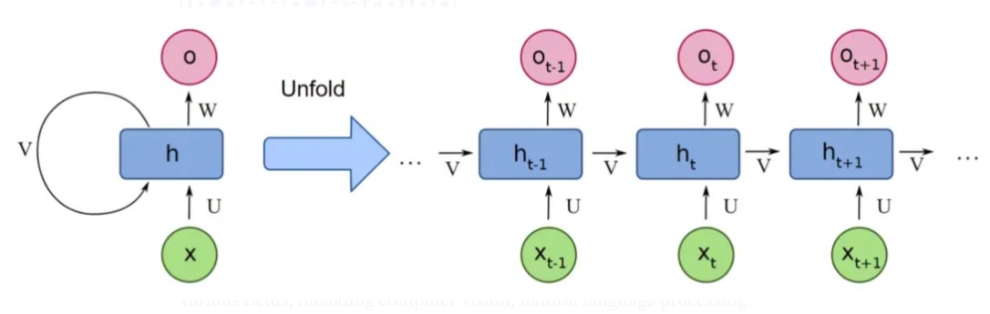
Architecture of RNNs

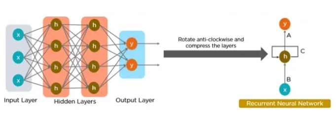
Recurrent Neural Networks (RNNs) are a type of neural network designed to process sequential data. Unlike classical networks (such as feedforward networks) that analyze each input independently, RNNs are able to retain information from the past to influence future predictions through feedback loops.

In some situations, such as predicting the next word in a sentence, it is essential to remember previous terms to generate a coherent response. Classical neural networks (without temporal memory) cannot handle these long-term dependencies, which motivated the creation of RNNs.

The Key Component: Hidden State 🧠

The hidden state acts as contextual memory, allowing RNNs to:

• Store relevant information from previous steps.
• Update memory at each time step.
• Influence future predictions through recurrent mechanisms.

📌 Main features of RNNs:

• They maintain a temporal context by memorizing key information from sequences.
• They apply the same parameters (weights) to each element of the sequence, thus reducing the complexity of the model (parameter sharing).
• They allow processing of sequential data such as text, audio, or time series, by exploiting their temporal structure.

Principal components of RNNs

a) Input Layer: The input layer of an RNN processes each element of the sequence (like a word in a sentence) by transforming it into a dense vector representation via embedding vectors. These embeddings, often pre-trained (like Word2Vec, GloVe, or BERT), are crucial because they:

• Capture semantic relationships between words (e.g., similarity, antonymy).
• Reduce dimensionality compared to a classic one-hot encoding.

For example, the words “cat” and “dog” (domestic animals) will have geometrically close vectors in the embedding space, unlike “cat” and “car”. This allows the RNN to:

• Understand analogies and lexical context.
• Generalize better on rare or unknown words.

This step is fundamental to analyzing linguistic or temporal sequences in a coherent manner, because it encodes the information before it is processed by the recurrent layers (hidden states).

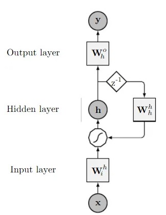
b) Hidden Layer: The hidden layer is the heart of an RNN, as it allows it to memorize the context and process data step by step. Unlike a classic neural network (like a feedforward), where inputs are processed in isolation, an RNN maintains a dynamic memory via its hidden state, a numerical vector that evolves at each step.

Two-Stage Operation

Each time step, the hidden layer receives:

• The current input (e.g., the word “beau” in the sentence “Il fait beau aujourd’hui”).
• The previous hidden state (a summary of the previous words, like “Il fait”).

These two elements are combined via an activation function (e.g., tanh or ReLU) to generate:

• A new hidden state (updated with the current context).
• An output (optional, depending on the task).

Concrete Example

In the sentence “It’s nice today”:

• When the RNN processes “beau”, the hidden state already contains the information “It’s nice”.
• This allows us to understand that “beau” describes the weather, and not an object (“un beau tableau”).

What is this memory used for?

• Machine translation: Connecting words from a source language to a target (“Chat” → “Cat” taking into account gender).
• Speech recognition: Deducing “ice cream” rather than “I scream” using the acoustic context.
• Text generation: Producing “Il fait froid” after “Il neige en hiver, donc…”.

Why is it revolutionary?

• Parameter sharing: The same weights are used at each time step (saving computation).
• Flexibility: Processes sequences of variable length (sentences, time series).

c) Activation function

The activation function is a critical component of an RNN, as it introduces non-linearity, enabling the network to learn complex relationships between elements in a sequence. Without this transformation, the RNN would process information linearly (like a basic calculator), limiting its ability to capture complex dependencies such as irony, intensity, or grammatical nuances.

How Does the Activation Function Work in an RNN?

At each timestep, a hidden layer neuron receives two inputs:

• Current input (e.g., a word in a sentence).
• Previous hidden state (a numerical summary of past elements).

These values are combined via a linear operation:

$h_t = W_x \cdot x_t + W_h \cdot h_{t-1} + b$

Issue: Without an activation function, this equation only allows proportional relationships (e.g., “twice as cold” = “twice as many clothes”), lacking contextual adaptation.

Solution: The activation function (e.g., tanh or ReLU) applies a non-linear transformation. This enables the RNN to:

• Capture conditional patterns (e.g., “very” amplifies “cold” but dampens “hot”).
• Dynamically modulate word impact based on context.

Why is Non-Linearity Necessary?

Without it, each hidden state h(t) would be a linear combination of past inputs. The RNN would then act like a simple statistical model, unable to:

• Differentiate between “It’s a bit cold” and “It’s very cold”.
• Distinguish “I love it!” (positive) from “I love it… not” (negative).

d) Output Layer

The output layer converts the final hidden state into a usable prediction:

Prediction conversion: Takes the last hidden state ht (full context) and converts it to:

• A word (e.g., next word in a translation).
• A class (e.g., “positive” or “negative” sentiment).
• A numerical value (e.g., predicted temperature).

Tailored activation functions:

• Softmax: For probabilities (e.g., choosing among 10,000 possible words).
• Sigmoid: For binary classification (e.g., spam vs. non-spam).
• Linear: For regression (e.g., stock price prediction).

Application example: Sentence: “It’s raining, so I’ll take my […]”

• Hidden state: Encodes context “rain” + “take”.
• Output layer → “umbrella” (using softmax).

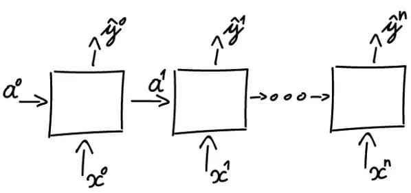
Different RNN Architectures

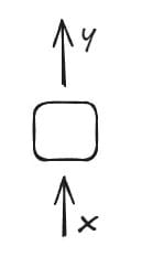
One-to-One Architecture

The One-to-One architecture is the simplest form, where a single input is mapped directly to a single output. This model lacks sequential processing or temporal dependencies, making it functionally similar to traditional neural networks (like a perceptron). It is often used as a baseline for comparing more complex RNN architectures (e.g., One-to-Many or Many-to-Many).

In this model:

• A single input (x) is processed to generate a single output (y).
• The output is computed using a linear mathematical function: $y=wx+b$

where:

• w: Weight (determines the input’s influence).
• b: Bias (offsets the prediction).

One-to-Many Architecture

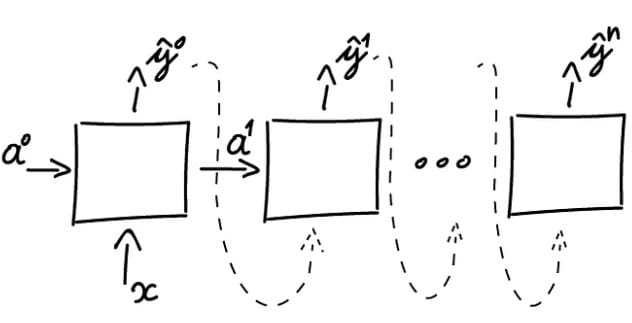The One-to-Many architecture is designed for scenarios where a single input generates a sequence of outputs. It excels in tasks requiring the transformation of a single data point into a structured, multi-step result.

How Does It Work?

a) Single Input (x): A single data point is fed into the network (e.g., an image, text prompt, or audio clip). b) Sequential Outputs (y₀, y₁, …, yₙ): The network generates outputs step-by-step, building a sequence over time.

c) Internal Propagation: At each step, the network uses:

• The previous hidden state (memory of past steps).
• The initial input or prior outputs to generate the next result.

This recurrence allows the model to maintain contextual coherence.

Concrete Examples

a) Text-to-Speech (TTS):

• Input: A text string (e.g., “Hello”).
• Output: A time-series audio waveform pronouncing the phrase.
• Mechanism: The RNN converts text into phonemes, then synthesizes audio frames sequentially.

b) Music Generation:

• Input: A seed note (e.g., C4) or genre tag (e.g., “jazz”).
• Output: A melody composed of multiple notes (e.g., [C4, E4, G4, …]).
• Mechanism: The RNN predicts note pitch, duration, and timing iteratively.

Many-to-One Architecture

In RNNs, the Many-to-One (N:1) architecture transforms a sequence of inputs into a single output. It is used to synthesize a sequence into a global value or category, such as:

• Sentiment Analysis: Determining the emotion of a text (“Positive/Negative”).
• Sequence Classification: Identifying abnormal patterns in time-series data.
• Time-Series Prediction: Estimating future values (e.g., stock prices).

Many-to-One Architecture Schema

Example: Sentiment analysis of the sentence “I loved this movie!”

Sequential Inputs:

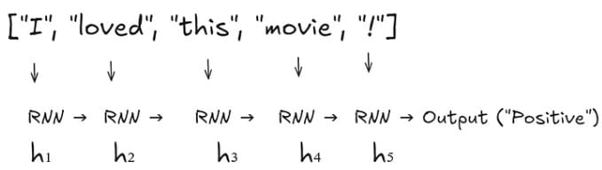
Detailed Propagation:

a) Input 1 (X₁ = “I”):

• Compute h₁:

  $h₁ = f(Wx·X₁ + Wh·h₀ + b)$

  (h₀ is initialized to zero or randomly)

b) Input 2 (X₂ = “loved”):

• Compute h₂:

  $h₂ = f(Wx·X₂ + Wh·h₁ + b)$

c) Input 5 (X₅ = ”!“):

• Compute h₅:

  $h₅ = f(Wx·X₅ + Wh·h₄ + b)$

  Output: $Y = softmax(Wy·h₅ + by)$ → “Positive”

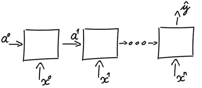
Many-to-Many Architecture

This architecture handles sequences where input and output lengths differ. It is split into two specialized components: an encoder and a decoder, enabling tasks like translation or text generation.

This architecture handles input and output sequences of different lengths.

Examples:

• Translation (“Bonjour” → “Hello”, “Comment ça va ?” → “How are you?”).
• Speech synthesis (text → audio).
• Dialogue systems (question → response).

Structure

Encoder

• Role: Transforms the input into a context (a vector of numbers).
• Function:
• Processes each input element (e.g., words in a sentence) one by one.
• Updates a hidden state (memory) at each step.
• The final hidden state (context) summarizes the entire input.

Decoder

• Role: Generates the output step by step, using the context.
• Function:
• Initializes its hidden state with the encoder’s context.
• Generates an output element (e.g., a word) at each timestep.
• Uses its own previous output as input for the next step (autoregression).

Advantages and Disadvantages of RNNs

Advantages of RNNs:

• Handle sequential data effectively, including text, speech, and time series.
• Process inputs of any length, unlike feedforward neural networks.
• Share weights across time steps, enhancing training efficiency.

Disadvantages of RNNs:

• Prone to vanishing and exploding gradient problems, hindering learning.
• Training can be challenging, especially for long sequences.
• Computationally slower than other neural network architectures.

What Are Different Variations of RNN?

Researchers have introduced new, advanced RNN architectures to overcome issues like vanishing and exploding gradients that hinder learning in long sequences.

• Long Short-Term Memory (LSTM): A popular choice for complex tasks. LSTM networks introduce gates, i.e., input gate, output gate, and forget gate, that control the flow of information within the network, allowing them to learn long-term dependencies more effectively than vanilla RNNs.

• Gated Recurrent Unit (GRU): Similar to LSTMs, GRUs use gates to manage information flow. However, they have a simpler architecture, making them faster to train while maintaining good performance. This makes them a good balance between complexity and efficiency.

• Bidirectional RNN: This variation processes data in both forward and backward directions. This allows it to capture context from both sides of a sequence, which is useful for tasks like sentiment analysis where understanding the entire sentence is crucial.

• Deep RNN: Stacking multiple RNN layers on top of each other, deep RNNs creates a more complex architecture. This allows them to capture intricate relationships within very long sequences of data. They are particularly useful for tasks where the order of elements spans long stretches.

Conclusion

Recurrent Neural Networks have revolutionized deep learning by enabling models to process sequential data effectively. Despite their limitations, advancements like LSTM, GRU, and Bidirectional RNNs have significantly improved their performance. However, modern architectures like Transformers are now pushing the boundaries of sequence modeling even further, marking the next evolution in AI-driven tasks.