Differents types of activation functions

Sigmoid Function

The sigmoid function is one of the most well-known activation functions in artificial intelligence and machine learning. It is defined by the following equation:

$f(x) = \frac{1}{1+e^{-x}}$

This function transforms any input value into a number between 0 and 1. Thanks to this property, it is often used to represent probabilities, making it an excellent choice for binary classification problems.

Limitations of the Sigmoid Function

Although the sigmoid function is useful, it has some drawbacks:

• Saturation Effect: For very large or very small input values, the output is close to 0 or 1, making the model less sensitive to variations.
• Vanishing Gradient Problem: In deep neural networks, the sigmoid function can cause slow learning, as gradients become too small.
• Non-Zero-Centered Output: Unlike other functions such as tanh, the sigmoid function produces only positive values (between 0 and 1). This can slow down model convergence because it forces the network’s weight updates to be unbalanced, making optimization less efficient.

Tanh Function

The Tanh function (or Hyperbolic Tangent) is an activation function used in neural networks. It transforms an input value into a number between -1 and 1.

Here is its mathematical formula:

$Tanh(x) = \frac{e^x-e^{-x}}{e^x+e^{-x}}$

This means that, no matter the value of x, the output of the function will always be between -1 and 1.

Why is it useful?

It centers values around zero Unlike the Sigmoid function, whose outputs are always positive (between 0 and 1), the Tanh function produces both positive and negative values (between -1 and 1).

• This helps neural networks learn more efficiently because positive and negative values are better balanced.
• It reduces the risk of the model being biased toward only positive values.

It helps normalize data By keeping values within a symmetric range (-1 to 1), Tanh allows for better weight adjustments in the neural network and accelerates learning.

RELU function

The ReLU (Rectified Linear Unit) function is one of the most widely used activation function in deep learning. It is mathematically defined as:

$f(x) = max(0,x) = \begin{cases} x_i, & \text{if } x_i \geq 0 \\ 0, & \text{if } x_i < 0 \end{cases}$

This means that:

• If x is positive, the function keeps it unchanged (i.e., f(x)=x).
• If x is negative or zero, the function outputs 0 (i.e., f(x)=0).

Why is ReLU useful?

Avoids the vanishing gradient problem

• In deep neural networks, activation functions like Sigmoid or Tanh can cause very small gradients during backpropagation, slowing down learning (this is called the vanishing gradient problem).
• Since ReLU does not squash large values, it allows gradients to stay strong, making training much faster and more efficient.

Computationally efficient

• ReLU is very simple to compute: it just requires checking whether the input is positive or not.
• This makes it much faster than other activation functions like Sigmoid or Tanh, which involve exponentials.

What is vanishing gradient?

Before talk about Vanishing gradient , let’s understand neural network weights and how to adjust them with backpropagation.

When training a neural network, such as a Convolutional Neural Network (CNN), the aim is to reduce the error between what the model predicts and what the actual data shows. This is achieved by adjusting the network’s weights. But what are these weights?

What are neural network weights? A neural network is made up of layers, each containing neurons. Each connection between these neurons is associated with a weight, which is simply a number. This weight determines the importance of a connection: a high weight means that the connection has a great influence, while a low weight means that the connection has little impact on the calculation.

During training, the network learns by modifying these weights to improve predictions. It’s a bit like adjusting the knobs on a radio to get clear sound: you adjust the weights to get the right prediction.

How Are Weights Adjusted?

To adjust the weights in a neural network, we use a method called backpropagation of the gradient (or simply Backpropagation). This process consists of three main steps:

1️⃣ Calculating the Error (Loss Function)

The first step is to measure the error between the model’s prediction and the actual value. This is done using a mathematical function called the Loss Function.

📌 Examples of Loss Functions:

• For a classification problem (e.g., predicting “dog” or “cat”), we often use Cross-Entropy Loss.
• For predicting continuous values (e.g., estimating a price), we use Mean Squared Error (MSE).

📌 Mathematical Example of Cross-Entropy Loss:

$Loss = -\sum_{i=1}^{\text{output size}} y_i \cdot \log \hat{y}_i$

where:

• **y(i)**​ is the true class label (e.g., “dog” or “cat”).
• ŷ(i) the predicted probability assigned to that class.

👉 This formula produces a value that represents the total error. The goal is to minimize this error as much as possible!

2️⃣ Computing the Gradient: Finding the Right Direction

Once the error is calculated, the model needs to adjust its weights to reduce it. But how do we know in which direction to change the weights? This is where the concept of gradient comes into play.

What is a Gradient?

A gradient is a mathematical measure that tells us how much and in which direction a value should change. In our case, it measures how the loss function changes with respect to each weight in the network.

📌 Mathematically, we compute the partial derivative of the loss function with respect to each weight:

📌 How do we interpret this?

• If the gradient is positive, we need to decrease the weight to reduce the error.
• If the gradient is negative, we need to increase the weight to reduce the error.
• If the gradient is close to zero, the weight stops changing significantly.

⚠️ This is where the Vanishing Gradient Problem occurs! When gradients become extremely small, the network struggles to update the weights in early layers, making learning very slow or even impossible

3️⃣ What is Backpropagation?

Backpropagation is a method used in neural networks to correct their errors. The main idea is to adjust the weights of the network (the “knobs” that control the strength of connections between neurons) so that the network makes better predictions next time.

• The network makes an error: When we give an input to the network (e.g., a picture of a cat), it produces an output (e.g., “dog” instead of “cat”). We compare this output to the correct answer to measure the error.

• Calculating how much each connection (weight) contributed to the error: We start by looking at the last layer (the one that gives the final answer) and compute how much each weight influenced the error. Then, we move backward layer by layer, adjusting the weights at each step.

• Using the gradient and the chain rule: When we adjust the weights, we need to understand how each weight influences the model’s error. To do this, we use the gradient, which tells us how much the error (or loss) changes with respect to each weight. The chain rule is a mathematical concept that allows us to compute this gradient efficiently, even when there are multiple layers in the network.

Imagine you need to understand how an action in a previous layer affected the final error. To do that, you have to trace how this action affects the next layer, and so on, until you reach the output. It’s like a domino effect, where each domino influences the one that follows it.

Here’s how we proceed:

• The final error (L) depends on the output of the network (O).
• The output (O) depends on the activation (H) of the previous layer.
• The activation (H) depends on the weights (W) of the layer.

By using the chain rule, we can combine these effects to calculate the impact of each weight on the final error.

Simple Chain Rule Formula: $\frac{\partial L}{\partial W_1} = \frac{\partial L}{\partial O} \times \frac{\partial O}{\partial H} \times \frac{\partial H}{\partial W_1}$

This means:

• ∂L/∂O​: Measures how much the error changes with respect to the output.
• ∂O/∂H​: Measures how much the output changes with respect to the activation of the previous layer.
• ∂H/∂W1​: Measures how much the activation changes with respect to the weight of the layer.

This cascade multiplication of gradients through the layers allows the network to understand the effect of each weight on the final error and adjust the weights accordingly. If a weight had a significant impact on the error, its gradient will be larger, and it will be adjusted more. If it had little impact, its gradient will be smaller, and it will be adjusted less.

• Updating the weights: Once we have computed the gradients, we update the weights to reduce the error. For example:

— If the gradient for a weight is positive, we decrease the weight.

— If the gradient is negative, we increase the weight.

— If the gradient is ** **, the weight stops changing significantly.

This process is repeated over many iterations (or epochs), with the weights being adjusted gradually, improving the network’s ability to make accurate predictions!

The Vanishing Gradient Problem occurs when gradients become very small (close to zero) in the early layers of the network. This means that the weights in these layers stop updating properly, causing the first layers to stop learning effectively.

Why does this happen?

Some activation functions, like Sigmoid or Tanh, have very small derivatives when their inputs are either very large or very small. This weakens the gradient as it propagates backward through the network.

Example with the Sigmoid Function The Sigmoid function is defined as:

$\sigma(x) = \frac{1}{1+e^{-x}}$

Its derivative is:

$\frac{d}{dx}\sigma(x) = \sigma(x)(1-\sigma(x))$

👉 When x is very large or very small, f(x) becomes close to 1 or 0, and its derivative approaches zero.

In a deep network, the gradient is computed layer by layer, multiplying these derivatives at each step.

• If the derivative is always small (<1), then gradients shrink with each multiplication.
• By the time they reach the earlier layers, they become almost zero → the first layers stop learning.

Why is this a problem?

🔴 The first layers stop learning → They remain unchanged and fail to capture basic features like edges and shapes.

🔴 Learning becomes very slow → Only the last layers (closer to the output) receive meaningful updates.

🔴 The network becomes ineffective → It struggles to learn complex patterns from the data.

How to Avoid the Vanishing Gradient?

✅ Use ReLU Instead of Sigmoid or Tanh 👉 The ReLU function is defined as:

f(x)=max⁡(0,x)

👉 Its derivative is 1 for positive values, meaning it does not shrink the gradient, preventing it from vanishing.

✅ Use Batch Normalization 👉 This technique normalizes the input values of each layer to prevent extreme values and stabilize learning, ensuring smoother training.

✅ Use Proper Weight Initialization (Xavier, He) 👉 Proper weight initialization prevents values from being too large or too small at the start, reducing the risk of activation saturation and gradient shrinkage.

✅ Use Advanced Optimizers (Adam, RMSprop) 👉 These optimization algorithms automatically adjust weight updates to prevent the gradient from becoming too small, ensuring efficient learning.

👉 Activation layers allow the network to model complex patterns instead of being limited to simple linear relationships. Once these complex features are extracted, pooling layers are used to reduce the data size while retaining the most important information. They act as a summary of the previous layers, making the network more efficient and less computationally demanding.

Pooling Layers

Pooling is an operation that reduces the size of feature maps while preserving key information. It works by grouping neighboring pixels and summarizing their content into a single value. This helps:

✅ Reduce data dimensions, speeding up computations.

✅ Preserve essential features (such as edges and contours).

✅ Increase model robustness against minor variations in an image (noise, shifts, and transformations).

How Does Pooling Work?

Pooling is a crucial step in convolutional neural networks (CNNs) used to reduce the size of data (images or feature maps) while retaining the most important information. Here’s how it works:

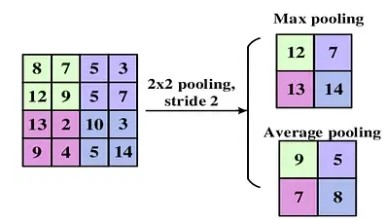
We define a small square region of the image (usually 2×2 or 3×3 pixels) and apply a pooling function to this region to compute a single value that represents it.

There are various types of pooling, each with unique advantages and use cases:

1️⃣ Max Pooling (The Most Common Type)

• How Does It Work? Max pooling selects the maximum value in the defined region.

• Why Use It? ✅ It captures the most prominent features of the image, such as edges and contours. ✅ It effectively preserves visually important details. ❌ However, it can be sensitive to noise: if an outlier pixel has a very high value, it will be retained.

📌 When to Use Max Pooling? ✅ When you want to keep the dominant structures of an image. ✅ Ideal for convolutional neural networks used in computer vision tasks (e.g., image classification, object detection).

2️⃣ Average Pooling

• How Does It Work? Average pooling calculates the mean of the values in the defined region.

• Why Use It?

✅ It smooths out variations and reduces the impact of extreme values. ✅ It is less sensitive to noise than max pooling. ❌ However, it may dilute important features like edges and contrasts.

📌 When to Use Average Pooling? ✅ When you want to reduce the size of the image without losing too much information. ✅ Suitable for tasks requiring smoother feature maps, such as speech recognition.

3️⃣ L2 Norm Pooling

How Does It Work? L2 Norm Pooling computes the L2 norm of the values in the region, which is the square root of the sum of squares of the values.

Why Use It? ✅ It provides a measure of the overall intensity of the region. ❌ It’s less commonly used than Max or Average Pooling but can be useful for specific tasks.

📌 When to Use L2 Norm Pooling? ✅ When you need a robust measure of pixel intensity, such as in industrial vision applications.

4️⃣ Weighted Average Pooling How Does It Work? Weighted Average Pooling computes a weighted mean, assigning more importance to central pixels in the region.

Why Use It? ✅ It is well-suited to images where the center contains the most critical information (e.g., in facial recognition). ❌ It is more computationally complex than other methods.

📌When to Use Weighted Average Pooling? ✅ When preserving central details of an image is important, such as in medical imaging (e.g., analyzing MRI scans).

How Pooling Fits into CNNs Pooling is typically applied after convolution and activation layers. Here’s how they work together:

• Convolution Layers extract features from the image by applying filters.
• Activation Layers (like ReLU) highlight important features by introducing non-linearity.
• Pooling Layers simplify the output by summarizing the most important information, reducing the data size and computational complexity.

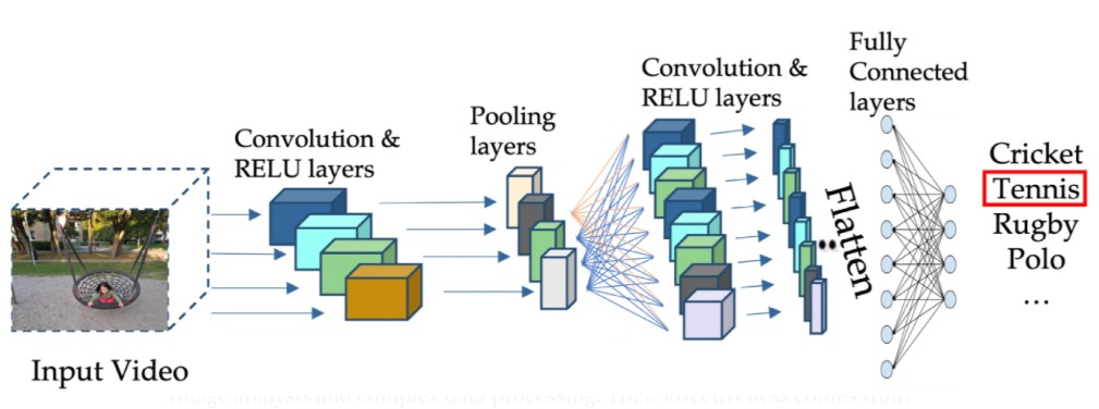
Flatten Layers

1️⃣ What is Flattening? Flattening is a simple but essential step in a Convolutional Neural Network (CNN). It is the process of transforming a 2D feature map into a 1D vector.

👉 Before Flattening: The data is in a 2D shape (Height × Width × Depth). 👉 After Flattening: The data becomes a long 1D vector, which can be fed into a traditional dense neural network layer.

2️⃣ Why is Flattening Necessary? Convolutional and pooling layers process images as matrices (2D or 3D). However, fully connected (dense) layers in a neural network expect a 1D vector as input.

✅ Flattening converts the feature map into a format that the fully connected layers can process.

Fully Connected Layers (FC)

Fully connected layers, also called dense layers, are a fundamental component of neural networks, especially in Convolutional Neural Networks (CNNs) and Deep Neural Networks (DNNs).

In a fully connected layer, every neuron is connected to all the neurons in the previous layer. This is in contrast to convolutional layers, where the connections are local and limited to small regions of the input (e.g., receptive fields).

Here’s how it works:

• Each neuron in the fully connected layer receives inputs from all the outputs of the previous layers.
• These inputs are multiplied by weights, and a bias is added.
• A non-linear activation function (like ReLU or Sigmoid) is then applied to produce the neuron’s output.

The fully connected layers combine all the extracted features from convolutional and pooling layers to produce the final decision of the network, whether it’s for classification (e.g., predicting a class label) or regression (e.g., outputting a continuous value).

Why are Fully Connected Layers Important? Fully connected layers play a key role in CNNs by:

• Taking the features extracted by convolutional and pooling layers.
• Combining them to produce a final output (e.g., probabilities of classes in classification tasks).
• Acting as the “brain” of the network, where all the information is synthesized for the final prediction.

Typically, fully connected layers appear at the end of a CNN and are used for tasks like classification or regression based on the processed information from earlier layers.

Now that we’ve covered the foundational components of CNNs, let’s move on to discuss Recurrent Neural Networks (RNNs) 👉