Introduction

Generative adversarial networks, or GANs, represent a cutting-edge approach to generative modeling in deep learning, often leveraging architectures such as convolutional neural networks. The goal of generative modeling is to autonomously identify patterns in the input data, allowing the model to produce new examples that realistically resemble the original dataset. GANs address this challenge through a unique setup, treating it as a supervised learning problem involving two key elements: the generator, which learns to produce new examples, and the discriminator, responsible for distinguishing between real and generated. Through adversarial training, these models engage in competitive interaction until the generator becomes adept at creating realistic samples, fooling the discriminator about half the time. This dynamic field of GANs has evolved rapidly, exhibiting remarkable capabilities in generating realistic content in various domains. Notable applications include image-to-image translation tasks and the creation of photorealistic images indistinguishable from real photos, demonstrating the transformative potential of GANs in the field of generative modeling.

What is GAN model?

GAN is a machine learning model in which two neural networks compete with each other by using deep learning methods to become more accurate in their predictions. GANs typically run unsupervised and use a cooperative zero-sum game framework to learn, where one person’s gain equals another person’s loss.

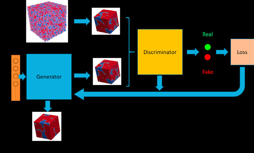
GANs consist of two models, namely, the generative model and the discriminator model. On the one hand, the generative model is responsible for creating fake data instances that resemble your training data. On the other hand, the discriminator model behaves as a classifier that distinguishes between real data instances from the output of the generator. The generator attempts to deceive the discriminator by generating real images as far as possible, and the discriminator tries to keep from being deceived.

The discriminator penalizes the generator for producing an absurd output. At the initial stages of the training process, the generator generates fake data, and the discriminator quickly learns to tell that it’s fake. But as the training progresses, the generator moves closer to producing an output that can fool the discriminator. Finally, if generator training goes well, then the discriminator performance gets worse because it can’t quickly tell the difference between real and fake. It starts to classify the fake data as real, and its accuracy decreases. Below is a picture of the whole system:

How does GAN Model works?

Building block of GAN are composed with 2 neural networks working together.

1. Generator: Model that learns to make fake things to look real

2. Discriminator: Model that learns to differentiate real from fake

The goal of generator is to fool the discriminator while discriminator’s goal is to distinguish betwen real from fake

The keep compete between each other until at the end fakes (generator by generator) look real (discriminator can’t differentiate).

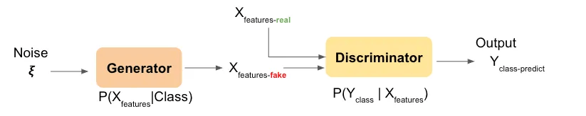We notice that what we input to generator is Noise, why? Noise in this scenario, we can think about it as random small number vector. When we vary the noise on each run(training), it helps ensure that generator will generate different image on the same class on the same class based on the data that feed into discriminator and got feed back to the generator.

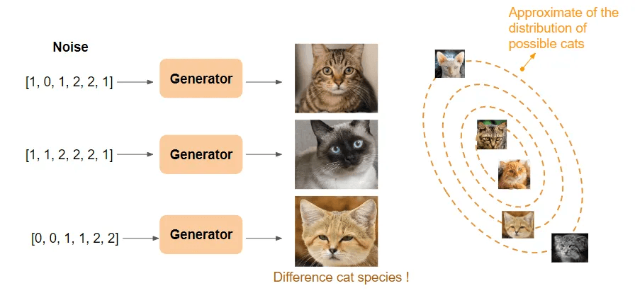
Then, generate will likely generate the object that are common to find features in the dataset. For example, 2 ears with round eye of cat rather with common color rather than sphinx cat image that might pretty be rare in the dataset.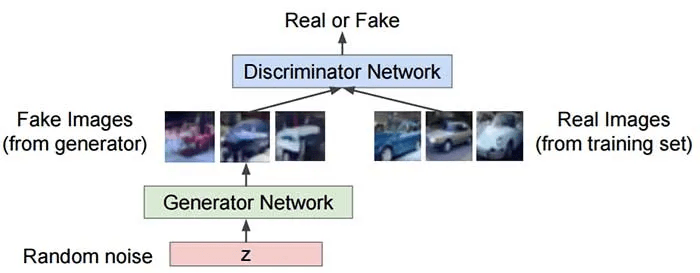

The generator model generated images from random noise(z) and then learns how to generate realistic images. Random noise which is input is sampled using uniform or normal distribution and then it is fed into the generator which generated an image. The generator output which are fake images and the real images from the training set is fed into the discriminator that learns how to differentiate fake images from real images. The output D(x) is the probability that the input is real. If the input is real, D(x) would be 1 and if it is generated, D(x) should be 0.

Metrics of GAN models

1. Kullback–Leibler and Jensen–Shannon Divergence

Let us talk about two metrics for quantifying the similarity between two probability distributions.

(1) KL (Kullback–Leibler) divergence measures how one probability distribution p diverges from a second expected probability distribution q.

$D_{KL}(p||q) = \int_x \mathrm{p(x)}log\frac{p(x)}{q(x)}d_{x}$

D(KL) achieves the minimum zero when p(x) == q(x) everywhere. It is noticeable according to the formula that KL divergence is asymmetric. In cases where p(x) is close to zero, but q(x) is significantly non-zero, the q’s effect is disregarded. It could cause buggy results when we just want to measure the similarity between two equally important distributions.

(2) Jensen–Shannon Divergence is another measure of similarity between two probability distributions, bounded by [0,1]. JS divergence is symmetric and more smooth.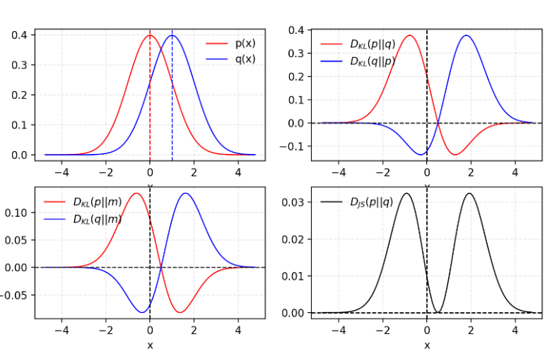

$D_{JS}(p||q) = \frac{1}{2}D_{KL}(p||\frac{p + q}{2}) + \frac{1}{2}D_{KL}(q||\frac{p + q}{2})$

Some believe (Huszar, 2015) that one reason behind GANs’ big success is switching the loss function from asymmetric KL divergence in traditional maximum-likelihood approach to symmetric JS divergence.

Small explanation about these metrics with examples

Let’s take the example of an image generator that creates images of cats. You have a generator that generates cat images, and you also have a set of real cat images.

The KL (Kullback-Leibler) divergence metric quantifies the difference between the distribution of images generated by the generator and the distribution of real images. Let’s assume you have two distributions: one corresponds to the distribution of images generated by the generator (let’s call it P), and the other corresponds to the distribution of real images (let’s call it Q). The KL divergence between P and Q measures how much information, on average, is needed to represent the differences between these two distributions. A higher value would indicate that the images generated by the generator are very different from the real images.

The KL divergence is not symmetric, which means that KL(P||Q) is not the same as KL(Q||P). This means that the way the generator approaches real images may be different from the way real images approach generated images. For example, it is possible for the generator to produce images that don’t resemble real images at all, while real images may have similarities with the generated images.

On the other hand, the Jensen-Shannon (JS) divergence is a symmetric measure that compares the similarity between the two distributions. It uses the KL divergence to calculate a symmetric similarity measure. In other words, the JS divergence between P and Q is the same as the JS divergence between Q and P. A JS divergence value close to zero would indicate that the images generated by the generator are very similar to the real images.

By using the JS divergence, you can evaluate the performance of your generator by measuring the similarity between the generated images and the real images. If the JS divergence is low, it means that the generator is capable of producing images that are similar to the real images. If the JS divergence is high, it indicates that the images generated by the generator are very different from the real images.

In summary, the KL divergence measures the difference between the distributions of generated and real images, while the JS divergence measures the similarity between these distributions. These measures help you evaluate the performance of your generator by comparing it to the real objects you want to generate.

2. EMD (earth’s mover distance) or Wassertein distance for WGAN model

The Earth Mover’s Distance (EMD) is a method to evaluate dissimilarity between two multi-dimensional distributions in some feature space where a distance measure between single features, which we call the ground distance is given.

The Wasserstein distance metric has several advantages over KL and JS divergences.

• First, it is more stable and often facilitates the convergence of GAN model training. It also makes it possible to better take into account mass differences between distributions, which can be useful when the distributions have different images or modes.

• The Wasserstein distance metric has an interesting geometric interpretation. It can be thought of as the minimum amount of work required to move mass from one distribution to another, where each unit of mass is considered a “pile of dirt” and the cost of moving is determined by a cost function. This geometric interpretation gives it interesting properties in terms of stability and convergence.

Small explanation about wasserstein metric with examples

Suppose you have a random number generator and you want to compare it to a real distribution of numbers. Your generator produces random numbers, but you want to know how similar these numbers are to those in the real distribution.

The KL divergence would tell you how different the two distributions are. It would measure the amount of additional information needed to represent the differences between the two distributions. For example, if your generator primarily produces numbers between 0 and 10, while the actual distribution is centered around 100, the KL divergence would be high to indicate that the two distributions are very different.

JS divergence, on the other hand, would tell you how similar the two distributions are. If your generator produces numbers that closely resemble those in the real distribution, the JS divergence would be small, indicating high similarity between the two distributions.

Now let’s look at the Wasserstein distance metric. She would tell you how much work is required to turn one distribution into another. In our example, this would mean how much effort you would have to put into transforming the distribution of numbers produced by your generator into the actual distribution of numbers. If the two distributions are very different, that would mean it would take a lot of work to make them similar.

To illustrate this, imagine that the actual distribution of numbers is a bell-shaped curve centered around 100. Your generator, on the other hand, mainly produces numbers between 0 and 10. The Wasserstein distance metric could tell you how many earth would need to be moved to transform the flat line between 0 and 10 into a curve of 100. The higher the Wasserstein distance metric, the more work would be required to perform this transformation. Look at the following figure to visualize what i am saying.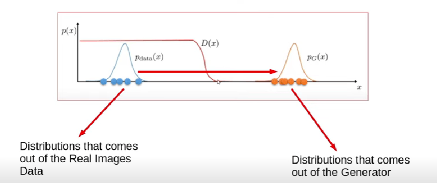

Types of GAN models

Deep Convolutional Generative Adversial Network

DCGAN stands for Deep Convolutional Generative Adversarial Network. It is a type of GAN that uses convolutional layers in both the generative and discriminative models.

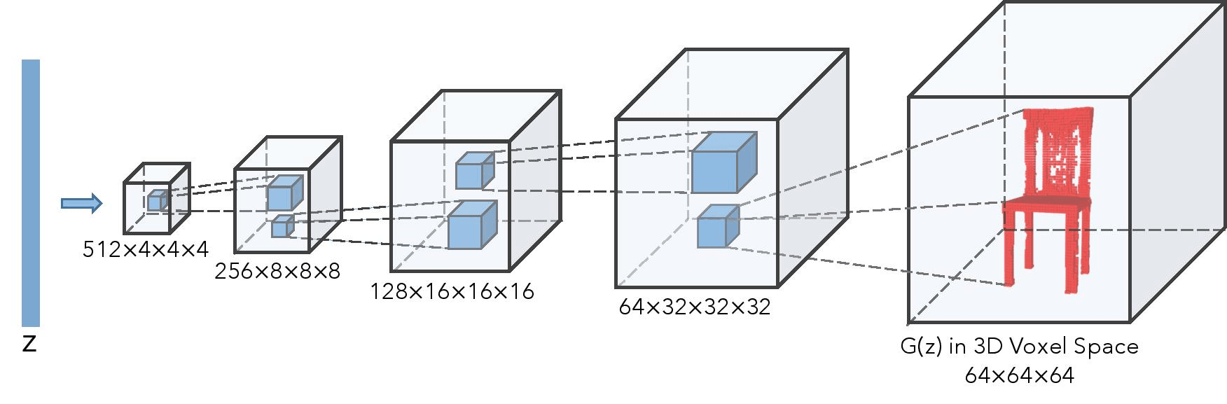
In a DCGAN, the generative model, G, is a deep convolutional neural network that takes as input a random noise vector, z, and outputs a synthetic image. The goal of G is to produce synthetic images that are similar to the real images in the training data. The discriminative model, D, is also a deep convolutional neural network that takes as input an image, either real or synthetic, and outputs a probability that the image is real. The goal of D is to correctly classify real images as real and synthetic images as fake.

The overall loss function for a DCGAN is defined as the sum of the loss functions for G and D. The loss function for G is defined as:

$L_G = E[log{(1 - D(G(z)))}]$

This loss function encourages G to produce synthetic images that are classified as real by D. In other words, it encourages G to generate images that are similar to the real images in the training data.

The loss function for D is defined as:

$L_G = E[log(D(x))] + E[log(1 - D(G(z)))]$

This loss function encourages D to correctly classify real images as real and synthetic images as fake. In other words, it encourages D to accurately differentiate between real and fake images.

The overall loss function for the DCGAN is then defined as:

$L_{DCGAN} = L_{G} + L_{D}$

This loss function is minimized during training by updating the weights of G and D using gradient descent. By minimizing this loss function, the DCGAN learns to generate high-quality synthetic images that are similar to the real images in the training data.

Wasserstein GAN

Wasserstein GANs (WGANs) are a type of Generative Adversarial Network (GAN) that use the Wasserstein distance (also known as the Earth Mover’s distance) as a measurement between the generated and real data distributions, providing several advantages over traditional GANs, which include improved stability and more reliable gradient information.

The architecture of a WGAN is not different than the traditional GAN, involving a generator network that produces fake images and a discriminator network that distinguishes between real and fake images. However, instead of using a binary output for the discriminator, a WGAN uses a continuous output that estimates the Wasserstein distance between the real and fake data distributions. During training, the generator is optimized to minimize the Wasserstein distance between the generated and real data distributions, while the discriminator is optimized to maximize this distance, leading to a more stable training process. It is worth mentioning that Wasserstein distance provides a smoother measure of distance than the binary cross-entropy used in traditional GANs.

One of the main advantages of WGANs is that they provide more reliable gradient information during training, helping to avoid problems such as vanishing gradients and mode collapse. In addition, the use of the Wasserstein distance provides a clearer measure of the quality of the generated images, as it directly measures the distance between the generated and real data distributions.

WGANs have been used in various applications, including image synthesis, image-to-image translation, and style transfer along with additional techniques such as gradient penalty, which improves stability and performance.

However, some challenges are associated with using WGANs, particularly related to the computation of the Wasserstein distance and the need for careful tuning of hyperparameters. There are also some limitations to the Wasserstein distance as a measure of distance between distributions, which can impact the model’s performance in certain situations.

CycleGANs

CycleGANs are a Generative Adversarial Network (GAN) used for image-to-image translation tasks, such as converting an image from one domain to another. Unlike traditional GANs, CycleGANs do not require paired training data, making them more flexible and easier to apply in real-world settings.

The architecture of a CycleGAN consists of two generators and two discriminators. One generator takes as input an image from one domain and produces an image in another domain whereas the other generator takes as input the generated image and produces an image in the original domain. The two discriminators are used to distinguish between real and fake images in each domain. During training, the generators are optimized to minimize the difference between the original image and the produced image by the other generator, while the discriminators are optimized to distinguish between real and fake images correctly. This process is repeated in both directions, creating a cycle between the two domains.

CycleGANs do not require paired training data which makes them more flexible and easier to apply in real-world settings. For example, they can be used to translate images from one style to another or generate synthetic images similar to real images in a particular domain.

CycleGANs have been used in various applications, including image style transfer, object recognition, and video processing. Additionally, they are also used to generate high-quality images from low-quality inputs, such as converting a low-resolution image to a high-resolution image.

However, CycleGANs come with certain challenges like complexity of the training process and the need for careful tuning of hyperparameters. In addition, there is a risk of mode collapse, where the generator produces a limited set of images that do not fully capture the diversity of the target domain.

Conclusion

In this article, we presented GANs, a new type of deep learning model capable of generating realistic contents such as images, text or video. After having defined the general operation of GANs composed of a generator and a discriminator confronting each other, we detailed some architectures such as basic GANs, conditional GANs or introspective GANs. We also looked at the main challenges related to unstable training of GANs, as well as their applications in areas like image synthesis or machine translation. Although perfectible, GANs open the way to creative artificial intelligence capable of generating new content autonomously. Future progress should enable ever more realistic generations and new innovative applications.